
 ついにWATLABブログから書籍「いきなりプログラミングPython」が発売しました!
波形の比較手段の一つとしてDTW(動的時間伸縮)をPythonでコーディングしていきます。ここでは理解を深めるために数式とフルスクラッチのPythonコードを使って説明します。また、最後に外部ライブラリであるlibrosaを使ったコード例も示します。
こんにちは。wat(@watlablog)です。ここでは波形の類似度を計算することができるDTWをPythonでやってみます!
DTWとは?
DTWとは、動的時間伸縮(Dynamic Time Warping)の略で、2つの時系列データの類似度を計算する手法です。WATLABブログでも過去に波形の相関を計算する記事を紹介していますが、リンク先の記事で紹介している手法はコサインの性質を利用して類似度を数値化するコサイン類似度と呼ばれる手法です。
・Pythonでベクトルと関数の相関を計算してみる
DTWはコサイン類似度よりも時間方向のデータのずれに頑健で、波形を扱うさまざまな分野で使用されています。DTWの説明は以下の英語版Wikiに載っている図や動画がわかりやすいと思うのでリンクを貼っておきます。
・Wiki:Dynamic Time Warping
この記事はDTWのアルゴリズムを理解するために、順を追ってPythonで実装しながら進めていきます。
動作環境
この記事のPythonは3.12.3で、外部ライブラリのバージョンはこちらです。
|
1 2 3 4 5 6 |
Package Version ------------------ ----------- librosa 0.11.0 matplotlib 3.10.3 numpy 2.2.6 pillow 11.2.1 |
DTWのフルスクラッチコード
時系列データの定義
この記事では、まず最初に簡単なサイン波を使ってDTWの基礎を学びます。波形の類似性を検証するために波形データは2つ用意します。波形のデータ形式は式(1)として用意します。
アルゴリズムの検証のために、データは振幅と周波数、位相の要素を変更できるよう式(2)でサイン波をつくります。
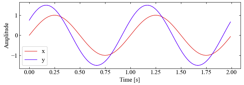
データをPythonでつくるとこんな感じです。matplotlibでグラフ化もしてみましょう。
|
1 2 3 4 5 6 7 8 9 10 11 12 13 14 15 16 17 18 19 20 21 22 23 24 25 26 27 28 29 30 31 32 33 34 35 36 37 38 39 40 41 42 43 44 45 46 47 48 49 50 |
import numpy as np import matplotlib.pyplot as plt def gen_wave(): """2つの波形を生成する関数""" # 波形諸元 a1 = 1 a2 = 1.5 f1 = 1 f2 = 1 phi1 = 0 phi2 = 30 t = np.arange(0, 2, 0.01) # 波形生成 x = a1 * np.sin(2 * np.pi * f1 * t + np.deg2rad(phi1)) y = a2 * np.sin(2 * np.pi * f2 * t + np.deg2rad(phi2)) return x, y, t def plot(x, y, t): """波形をプロットする関数""" # matplotlibの設定 plt.rcParams['font.size'] = 14 plt.rcParams['font.family'] = 'Times New Roman' plt.rcParams['xtick.direction'] = 'in' plt.rcParams['ytick.direction'] = 'in' fig, ax = plt.subplots(figsize=(8, 3)) ax.yaxis.set_ticks_position('both') ax.xaxis.set_ticks_position('both') ax.set_xlabel('Time [s]') ax.set_ylabel('Amplitude') # 波形データをプロット ax.plot(t, x, lw=1, color='red', label='x') ax.plot(t, y, lw=1, color='blue', label='y') ax.legend() fig.tight_layout() plt.show() return if __name__ == "__main__": """メイン""" #データ生成 x, y, t= gen_wave() plot(x, y, t) |
上記Pythonコードを実行すると周波数は同じで振幅と位相が異なる2つの波形がプロットされます。
局所コスト行列
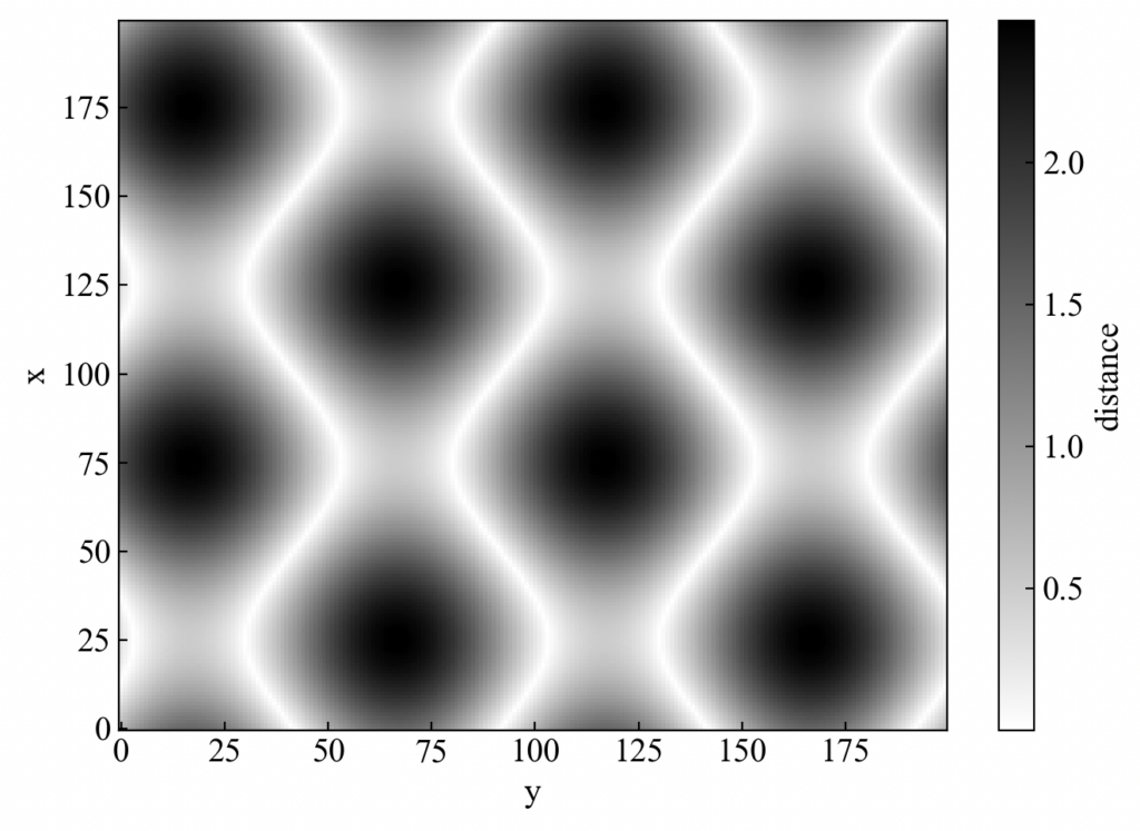
DTWは\(n\)個の\(x\)と\(m\)個の\(y\)でマトリクスをつくり、それぞれの波形要素同士で距離を計算する距離関数を用います。距離には色々な定義がありますが、ここではユークリッド距離を用いて説明します。距離関数を用いて各波形要素同士の計算を行うと、距離関数の行列ができます。これを局所コスト行列と呼び、式(3)で表現されます。
局所コスト行列の計算と2Dプロットまで行うPythonコードはこちらです。先ほど上の方で書いていた波形プロットウィンドウを消すと2Dプロット(白いほど距離が近い)が表示されます。
|
1 2 3 4 5 6 7 8 9 10 11 12 13 14 15 16 17 18 19 20 21 22 23 24 25 26 27 28 29 30 31 32 33 34 35 36 37 38 39 40 41 42 43 44 45 46 47 48 49 50 51 52 53 54 55 56 57 58 59 60 61 62 63 64 65 66 67 68 69 70 71 |
import numpy as np import matplotlib.pyplot as plt def gen_wave(): """2つの波形を生成する関数""" # 波形諸元 a1 = 1 a2 = 1.5 f1 = 1 f2 = 1 phi1 = 0 phi2 = 30 t = np.arange(0, 2, 0.01) # 波形生成 x = a1 * np.sin(2 * np.pi * f1 * t + np.deg2rad(phi1)) y = a2 * np.sin(2 * np.pi * f2 * t + np.deg2rad(phi2)) return x, y, t def local_cost_matrix(x, y): """ユークリッド距離による局所コスト行列を計算する関数""" return np.sqrt((x[:, None] - y[None, :])**2) def plot(x, y, t): """波形をプロットする関数""" # matplotlibの設定 plt.rcParams['font.size'] = 14 plt.rcParams['font.family'] = 'Times New Roman' plt.rcParams['xtick.direction'] = 'in' plt.rcParams['ytick.direction'] = 'in' fig, ax = plt.subplots(figsize=(8, 3)) ax.yaxis.set_ticks_position('both') ax.xaxis.set_ticks_position('both') ax.set_xlabel('Time [s]') ax.set_ylabel('Amplitude') # 波形データをプロット ax.plot(t, x, lw=1, color='red', label='x') ax.plot(t, y, lw=1, color='blue', label='y') ax.legend() fig.tight_layout() plt.show() return def plot2d(D): """行列グレースケールで表示する関数""" fig, ax = plt.subplots(figsize=(7, 5)) c = ax.imshow(D, origin='lower', aspect='auto', cmap='gray_r') ax.set_xlabel('y') ax.set_ylabel('x') fig.colorbar(c, ax=ax, label='distance') fig.tight_layout() plt.show() return if __name__ == "__main__": """メイン""" # データ生成 x, y, t= gen_wave() plot(x, y, t) # 局所コスト関数の計算 D = local_cost_matrix(x, y) plot2d(D) |
局所コスト行列のプロット結果がこちらです。計算結果をそのままプロットすると行列の縦が\(x\)になります。基礎的な学習はデータの形を確かめるのが重要です。\(x\)か\(y\)のデータに[:50]等でスライスすることでデータのサイズを変更できますが、片方だけスライスしてみる等でデータ形式の検証ができます。
今回はサイン波同士の計算であるため距離の近い(白い)部分は周期的に現れていることがわかります。
累積コスト行列(グローバルコスト行列)
続いて累積コスト行列を求めます。累積コスト行列とは、局所コスト行列\(D\)を使って「これまでの最小コストを積み上げた」行列を指しグローバルコスト行列\(C\)とも呼ばれます。
局所コスト行列が既知(\(D \in \mathbb{R}^{n \times m}\))とすると、累積コスト行列\(C\)は次の式(4)〜式(6)で示されます。
\(\in \mathbb{R}^{n \times m}\)は実数全体\(n \times m\)行列の集合空間の要素である、ことを意味していて、「\(n\)行\(m\)列の実数行列である」ということですね。
式(4)は前提条件です。コストの計算は必ず行列の[1,1]から始まるように設定します。後ほどこの左下のセルから始まるワーピングパスの計算を行います。
行列の1行目と1列目は式(5)で累積計算します。
式(6)は\(i \geq 2, j \geq 2\)の場合の計算式で、縦横斜めのいずれの経路から来ても最小となるものを選びます。これを再帰的に繰り返しますが、このような複雑な最適化問題を小さな部分問題に分割してその解を利用しながら効率的に解く方法を動的計画法と呼びます。
累積コスト行列を計算するPythonコードを示します。
|
1 2 3 4 5 6 7 8 9 10 11 12 13 14 15 16 17 18 19 20 21 22 23 24 25 26 27 28 29 30 31 32 33 34 35 36 37 38 39 40 41 42 43 44 45 46 47 48 49 50 51 52 53 54 55 56 57 58 59 60 61 62 63 64 65 66 67 68 69 70 71 72 73 74 75 76 77 78 79 80 81 82 83 84 85 86 87 88 89 90 91 92 93 94 95 96 97 98 99 |
import numpy as np import matplotlib.pyplot as plt def gen_wave(): """2つの波形を生成する関数""" # 波形諸元 a1 = 1 a2 = 1.5 f1 = 1 f2 = 1 phi1 = 0 phi2 = 30 t = np.arange(0, 2, 0.01) # 波形生成 x = a1 * np.sin(2 * np.pi * f1 * t + np.deg2rad(phi1)) y = a2 * np.sin(2 * np.pi * f2 * t + np.deg2rad(phi2)) return x, y, t def local_cost_matrix(x, y): """ユークリッド距離による局所コスト行列を計算する関数""" return np.sqrt((x[:, None] - y[None, :])**2) def global_cost_matrix(D): """累積コスト行列を計算する関数""" n, m = D.shape C = np.zeros((n, m), dtype=D.dtype) # 初期条件 C[0, 0] = D[0, 0] for i in range(1, n): C[i, 0] = D[i, 0] + C[i-1, 0] for j in range(1, m): C[0, j] = D[0, j] + C[0, j-1] # 再帰関係 for i in range(1, n): for j in range(1, m): C[i, j] = D[i, j] + min( C[i-1, j], C[i, j-1], C[i-1, j-1] ) return C def plot(x, y, t): """波形をプロットする関数""" # matplotlibの設定 plt.rcParams['font.size'] = 14 plt.rcParams['font.family'] = 'Times New Roman' plt.rcParams['xtick.direction'] = 'in' plt.rcParams['ytick.direction'] = 'in' fig, ax = plt.subplots(figsize=(8, 3)) ax.yaxis.set_ticks_position('both') ax.xaxis.set_ticks_position('both') ax.set_xlabel('Time [s]') ax.set_ylabel('Amplitude') # 波形データをプロット ax.plot(t, x, lw=1, color='red', label='x') ax.plot(t, y, lw=1, color='blue', label='y') ax.legend() fig.tight_layout() plt.show() return def plot2d(D): """行列グレースケールで表示する関数""" fig, ax = plt.subplots(figsize=(7, 5)) c = ax.imshow(D, origin='lower', aspect='auto', cmap='gray_r') ax.set_xlabel('y') ax.set_ylabel('x') fig.colorbar(c, ax=ax, label='distance') fig.tight_layout() plt.show() return if __name__ == "__main__": """メイン""" # データ生成 x, y, t= gen_wave() plot(x, y, t) # 局所コスト関数の計算 D = local_cost_matrix(x, y) plot2d(D) # グローバルコスト行列の計算 C = global_cost_matrix(D) plot2d(C) |
このコードを実行すると、ぼやっと斜めに白くなる2Dプロットを得ます。
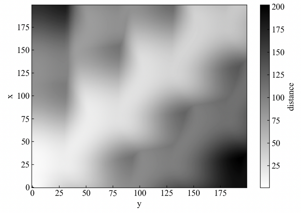
すでに人間の目には最適なワーピングパスが見える…かな?
最適ワーピングパスの探索
ワーピングパスとは、以下の制約を持つ経路のことで、1次元の順序集合\(p=(p_{1},p_{2},\dots, p_{k})\)で表現します。
- 境界条件:始点は[1, 1]、終点は[\(n\), \(m\)]である(式(7))。
パスの始点と終点が規定されることで、各データ内要素すべてを経路対象として保証します。
- 単調性:パスが進む毎に必ずインデックス(時間)が進む(式(8))。
DTWで自然なずらし合わせができる所以がここにあります。この式では行列のそれぞれのインデックスが「増えるか」「同じか」を意味しており、逆に戻ることはない(-1を許容しない)という特性を持ちます。この特性を単調性(Monotonicity)と呼びます。
- ステップサイズ制約:次のステップへは縦横斜めに1つのみ(式(9))。
上記単調性と共にステップサイズが固定になることで大ジャンプを防ぎます。これは局所的な連続性が保たれることを意味します。
ワーピングパスを計算するPythonコードを以下に示します。
|
1 2 3 4 5 6 7 8 9 10 11 12 13 14 15 16 17 18 19 20 21 22 23 24 25 26 27 28 29 30 31 32 33 34 35 36 37 38 39 40 41 42 43 44 45 46 47 48 49 50 51 52 53 54 55 56 57 58 59 60 61 62 63 64 65 66 67 68 69 70 71 72 73 74 75 76 77 78 79 80 81 82 83 84 85 86 87 88 89 90 91 92 93 94 95 96 97 98 99 100 101 102 103 104 105 106 107 108 109 110 111 112 113 114 115 116 117 118 119 120 121 122 123 124 125 126 127 128 129 130 131 132 133 134 135 136 137 138 139 140 141 142 143 144 |
import numpy as np import matplotlib.pyplot as plt def gen_wave(): """2つの波形を生成する関数""" # 波形諸元 a1 = 1 a2 = 1.5 f1 = 1 f2 = 1 phi1 = 0 phi2 = 30 t = np.arange(0, 2, 0.01) # 波形生成 x = a1 * np.sin(2 * np.pi * f1 * t + np.deg2rad(phi1)) y = a2 * np.sin(2 * np.pi * f2 * t + np.deg2rad(phi2)) return x, y, t def local_cost_matrix(x, y): """ユークリッド距離による局所コスト行列を計算する関数""" return np.sqrt((x[:, None] - y[None, :])**2) def global_cost_matrix(D): """累積コスト行列を計算する関数""" n, m = D.shape C = np.zeros((n, m), dtype=D.dtype) # 初期条件 C[0, 0] = D[0, 0] for i in range(1, n): C[i, 0] = D[i, 0] + C[i-1, 0] for j in range(1, m): C[0, j] = D[0, j] + C[0, j-1] # 再帰関係 for i in range(1, n): for j in range(1, m): C[i, j] = D[i, j] + min( C[i-1, j], C[i, j-1], C[i-1, j-1] ) return C def warping_path(C): """ワーピングパスを計算する関数""" n, m = C.shape i, j = n-1, m-1 path = [(i, j)] # (0,0) になるまで逆追跡 while (i > 0) or (j > 0): # 候補セルとそのコストをリスト化 candidates = [] if i > 0 and j > 0: candidates.append(((i-1, j-1), C[i-1, j-1])) if i > 0: candidates.append(((i-1, j), C[i-1, j])) if j > 0: candidates.append(((i, j-1), C[i, j-1])) # 最小コストの候補を選択 (i, j), _ = min(candidates, key=lambda x: x[1]) path.append((i, j)) return path[::-1] def plot(x, y, t): """波形をプロットする関数""" # matplotlibの設定 plt.rcParams['font.size'] = 14 plt.rcParams['font.family'] = 'Times New Roman' plt.rcParams['xtick.direction'] = 'in' plt.rcParams['ytick.direction'] = 'in' fig, ax = plt.subplots(figsize=(8, 3)) ax.yaxis.set_ticks_position('both') ax.xaxis.set_ticks_position('both') ax.set_xlabel('Time [s]') ax.set_ylabel('Amplitude') # 波形データをプロット ax.plot(t, x, lw=1, color='red', label='x') ax.plot(t, y, lw=1, color='blue', label='y') ax.legend() fig.tight_layout() plt.show() return def plot2d(D): """行列をグレースケールで表示する関数""" fig, ax = plt.subplots(figsize=(7, 5)) c = ax.imshow(D, origin='lower', aspect='auto', cmap='gray_r') ax.set_xlabel('y') ax.set_ylabel('x') fig.colorbar(c, ax=ax, label='distance') fig.tight_layout() plt.show() return def plot2d_with_warping_path(C, path): """行列をグレースケールで表示してワーピングパスを描画する関数""" fig, ax = plt.subplots(figsize=(7, 5)) c = ax.imshow(C, origin='lower', aspect='auto', cmap='gray_r') ax.set_xlabel('y') ax.set_ylabel('x') fig.colorbar(c, ax=ax, label='distance') ys, xs = zip(*path) ax.plot(xs, ys,linewidth=2, color='blue', label='Warping Path') fig.tight_layout() plt.show() return if __name__ == "__main__": """メイン""" # データ生成 x, y, t= gen_wave() plot(x, y, t) # 局所コスト関数の計算 D = local_cost_matrix(x, y) plot2d(D) # グローバルコスト行列の計算 C = global_cost_matrix(D) plot2d(C) # ワーピングパスの計算 path = warping_path(C) plot2d_with_warping_path(C, path) |
得られたワーピングパスを累積コスト行列の上に描画すると、次のプロットを得ます。
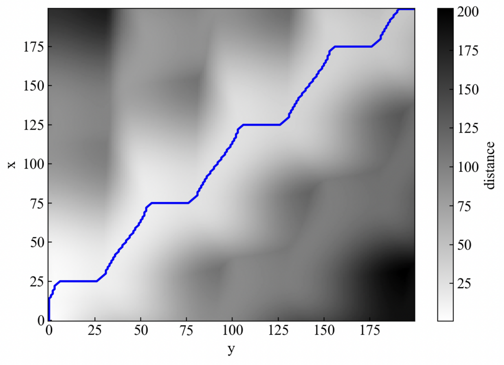
これでワーピングパスが決定されました!
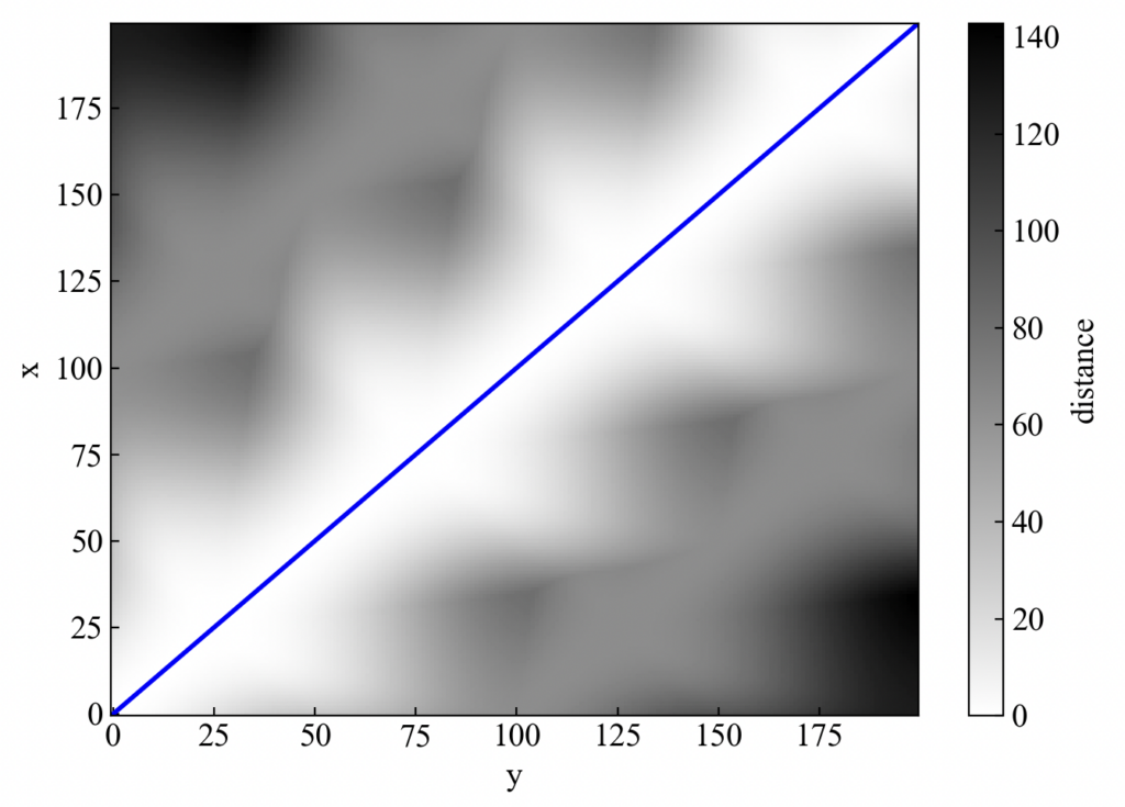
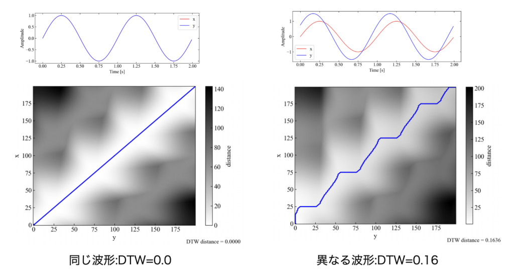
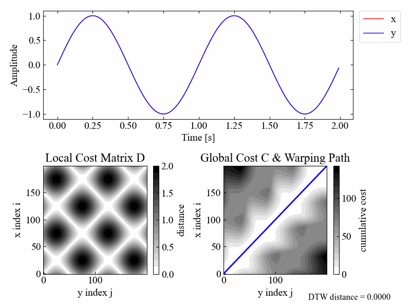
ちなみに、振幅a2=1, 位相phi2=0として2つの波形をまったく同じにすると、次の絵になります。波形の長さもサンプリングも一緒であるため、綺麗な斜め45度線が確認できました(迷いのないパス)。
DTW距離
時系列データ\(x\)と\(y\)がどれだけ似ているかはDTW距離という指標で評価できます。DTW距離は単純に累積コスト行列のワーピングパス終端数値です。パスの長さ\(k\)を使って正規化するとDTW距離は式(10)で示されます。
DTW距離は波形がまったく同じ場合は0になります(下図それぞれのプロット右下に計算結果を記載)。
色々な波形変化で結果を観察してみる
下準備(コードを見やすくする)
ここまででDTWの概要は説明完了です。あとは波形の素性をいじって遊んでみましょう!その前に、現状のコードはプロットウィンドウをいちいち消してからワーピングパスの確認までしていたので、まずはこのプロットをまとめるコードに変更します。さらに、次のコードでワーピングパスの情報を使って時系列波形のどことどこが対応するかも可視化してみましょう。
|
1 2 3 4 5 6 7 8 9 10 11 12 13 14 15 16 17 18 19 20 21 22 23 24 25 26 27 28 29 30 31 32 33 34 35 36 37 38 39 40 41 42 43 44 45 46 47 48 49 50 51 52 53 54 55 56 57 58 59 60 61 62 63 64 65 66 67 68 69 70 71 72 73 74 75 76 77 78 79 80 81 82 83 84 85 86 87 88 89 90 91 92 93 94 95 96 97 98 99 100 101 102 103 104 105 106 107 108 109 110 111 112 113 114 115 116 117 118 119 120 121 122 123 124 125 126 127 128 129 130 131 132 133 134 135 136 137 138 139 140 141 142 143 144 145 146 147 148 149 150 151 152 153 154 155 156 |
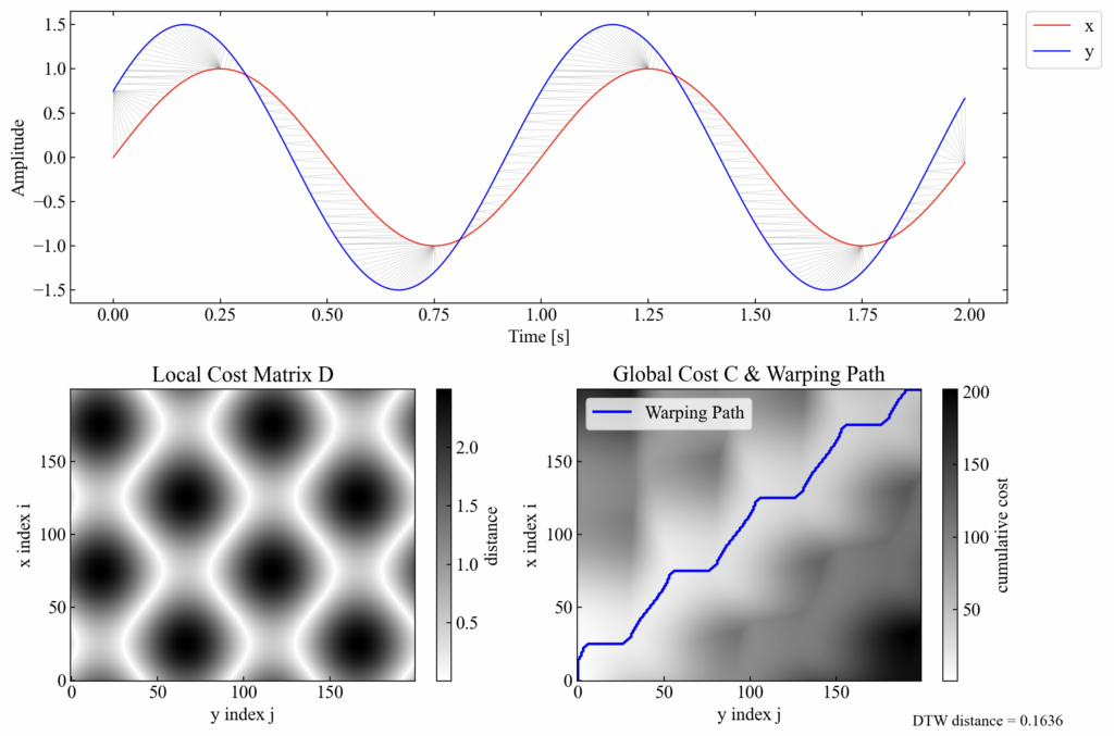
import numpy as np import matplotlib.pyplot as plt def gen_wave(): """2つの波形を生成する関数""" # 波形諸元 a1 = 1 a2 = 1.5 f1 = 1 f2 = 1 phi1 = 0 phi2 = 30 t = np.arange(0, 2, 0.01) # 波形生成 x = a1 * np.sin(2 * np.pi * f1 * t + np.deg2rad(phi1)) y = a2 * np.sin(2 * np.pi * f2 * t + np.deg2rad(phi2)) return x, y, t def local_cost_matrix(x, y): """ユークリッド距離による局所コスト行列を計算する関数""" return np.sqrt((x[:, None] - y[None, :])**2) def global_cost_matrix(D): """累積コスト行列を計算する関数""" n, m = D.shape C = np.zeros((n, m), dtype=D.dtype) # 初期条件 C[0, 0] = D[0, 0] for i in range(1, n): C[i, 0] = D[i, 0] + C[i-1, 0] for j in range(1, m): C[0, j] = D[0, j] + C[0, j-1] # 再帰関係 for i in range(1, n): for j in range(1, m): C[i, j] = D[i, j] + min( C[i-1, j], C[i, j-1], C[i-1, j-1] ) return C def warping_path(C): """ワーピングパスを計算する関数""" n, m = C.shape i, j = n-1, m-1 path = [(i, j)] # (0,0) になるまで逆追跡 while (i > 0) or (j > 0): # 候補セルとそのコストをリスト化 candidates = [] if i > 0 and j > 0: candidates.append(((i-1, j-1), C[i-1, j-1])) if i > 0: candidates.append(((i-1, j), C[i-1, j])) if j > 0: candidates.append(((i, j-1), C[i, j-1])) # 最小コストの候補を選択 (i, j), _ = min(candidates, key=lambda x: x[1]) path.append((i, j)) return path[::-1] def plot_all(x, y, t, D, C, path, dtw_distance): """全プロットをまとめる関数""" # matplotlibの設定 plt.rcParams['font.size'] = 14 plt.rcParams['font.family'] = 'Times New Roman' plt.rcParams['xtick.direction'] = 'in' plt.rcParams['ytick.direction'] = 'in' fig = plt.figure(figsize=(12, 8)) gs = fig.add_gridspec(2, 2, height_ratios=[1, 1]) # 上段:波形プロット(2列分を使用) ax_wave = fig.add_subplot(gs[0, :]) ax_wave.yaxis.set_ticks_position('both') ax_wave.xaxis.set_ticks_position('both') ax_wave.plot(t, x, lw=1, color='red', label='x') ax_wave.plot(t, y, lw=1, color='blue', label='y') # ワーピングパスに基づいて対応点同士を線で結ぶ for i, j in path: ax_wave.plot( [t[i], t[j]], [x[i], y[j]], color='gray', alpha=0.3, linewidth=0.5, zorder=0 ) ax_wave.set_xlabel('Time [s]') ax_wave.set_ylabel('Amplitude') ax_wave.legend(loc='upper left', bbox_to_anchor=(1.02, 1), borderaxespad=0) # 下段左:局所コスト行列 D ax_d = fig.add_subplot(gs[1, 0]) im_d = ax_d.imshow(D, origin='lower', aspect='auto', cmap='gray_r') ax_d.set_title('Local Cost Matrix D') ax_d.set_xlabel('y index j') ax_d.set_ylabel('x index i') fig.colorbar(im_d, ax=ax_d, label='distance') # 下段右:累積コスト行列 C + ワーピングパス + DTW距離 ax_c = fig.add_subplot(gs[1, 1]) im_c = ax_c.imshow(C, origin='lower', aspect='auto', cmap='gray_r') ys, xs = zip(*path) ax_c.plot(xs, ys, linewidth=2, color='blue', label='Warping Path') ax_c.set_title('Global Cost C & Warping Path') ax_c.set_xlabel('y index j') ax_c.set_ylabel('x index i') ax_c.legend(loc='upper left') fig.colorbar(im_c, ax=ax_c, label='cumulative cost') # 図全体の下部に DTW距離テキスト fig.text( 0.95, 0.02, f'DTW distance = {dtw_distance:.4f}', ha='right', va='bottom', fontsize=12 ) fig.tight_layout() plt.show() return if __name__ == "__main__": """メイン""" # データ生成 x, y, t= gen_wave() # 局所コスト関数の計算 D = local_cost_matrix(x, y) # グローバルコスト行列の計算 C = global_cost_matrix(D) # ワーピングパスの計算(DTW距離) path = warping_path(C) dtw_distance = C[-1, -1] / len(path) # プロット plot_all(x, y, t, D, C, path, dtw_distance) |
下図が実行結果です。これまで学んできた各プロットが全部まとまりました。さらに、ワーピングパスの情報から時間波形上で対応部分の線分を描画することで、ワーピングパスの屈曲点と線の密集具合が対応していることもわかりやすくなったと思います。
位相変化
まずは位相の変化をみてみましょう。サイン波形\(y\)の位相を360°分変化させ、動画として保存するために、上記Pythonコードをさらに次のように変更します。
GIF動画の作り方はWATLABブログの過去記事から引用しました。
・Pythonで複数画像からGIFを作る時に便利な処理まとめ
|
1 2 3 4 5 6 7 8 9 10 11 12 13 14 15 16 17 18 19 20 21 22 23 24 25 26 27 28 29 30 31 32 33 34 35 36 37 38 39 40 41 42 43 44 45 46 47 48 49 50 51 52 53 54 55 56 57 58 59 60 61 62 63 64 65 66 67 68 69 70 71 72 73 74 75 76 77 78 79 80 81 82 83 84 85 86 87 88 89 90 91 92 93 94 95 96 97 98 99 100 101 102 103 104 105 106 107 108 109 110 111 112 113 114 115 116 117 118 119 120 121 122 123 124 125 126 127 128 129 130 131 132 133 134 135 136 137 138 139 140 141 142 143 144 145 146 147 148 149 150 151 152 153 154 155 156 157 158 159 160 161 162 163 164 165 166 167 168 169 170 171 172 173 174 175 176 177 178 179 180 181 182 183 184 |
import numpy as np import matplotlib.pyplot as plt import os import glob from PIL import Image def gen_wave(a1=1, a2=1, f1=1, f2=1, phi1=0, phi2=0, duration=2, dt=0.01): """2つの波形を生成する関数""" # 波形生成 t = np.arange(0, duration, dt) x = a1 * np.sin(2 * np.pi * f1 * t + np.deg2rad(phi1)) y = a2 * np.sin(2 * np.pi * f2 * t + np.deg2rad(phi2)) return x, y, t def local_cost_matrix(x, y): """ユークリッド距離による局所コスト行列を計算する関数""" return np.sqrt((x[:, None] - y[None, :])**2) def global_cost_matrix(D): """累積コスト行列を計算する関数""" n, m = D.shape C = np.zeros((n, m), dtype=D.dtype) # 初期条件 C[0, 0] = D[0, 0] for i in range(1, n): C[i, 0] = D[i, 0] + C[i-1, 0] for j in range(1, m): C[0, j] = D[0, j] + C[0, j-1] # 再帰関係 for i in range(1, n): for j in range(1, m): C[i, j] = D[i, j] + min( C[i-1, j], C[i, j-1], C[i-1, j-1] ) return C def warping_path(C): """ワーピングパスを計算する関数""" n, m = C.shape i, j = n-1, m-1 path = [(i, j)] # (0,0) になるまで逆追跡 while (i > 0) or (j > 0): # 候補セルとそのコストをリスト化 candidates = [] if i > 0 and j > 0: candidates.append(((i-1, j-1), C[i-1, j-1])) if i > 0: candidates.append(((i-1, j), C[i-1, j])) if j > 0: candidates.append(((i, j-1), C[i, j-1])) # 最小コストの候補を選択 (i, j), _ = min(candidates, key=lambda x: x[1]) path.append((i, j)) return path[::-1] def plot_all(x, y, t, D, C, path, dtw_distance, filename): """全プロットをまとめる関数""" # matplotlibの設定 plt.rcParams['font.size'] = 14 plt.rcParams['font.family'] = 'Times New Roman' plt.rcParams['xtick.direction'] = 'in' plt.rcParams['ytick.direction'] = 'in' fig = plt.figure(figsize=(8, 6)) gs = fig.add_gridspec(2, 2, height_ratios=[1, 1]) # 上段:波形プロット(2列分を使用) ax_wave = fig.add_subplot(gs[0, :]) ax_wave.yaxis.set_ticks_position('both') ax_wave.xaxis.set_ticks_position('both') ax_wave.plot(t, x, lw=1, color='red', label='x') ax_wave.plot(t, y, lw=1, color='blue', label='y') # ワーピングパスに基づいて対応点同士を線で結ぶ for i, j in path: ax_wave.plot( [t[i], t[j]], [x[i], y[j]], color='gray', alpha=0.3, linewidth=0.5, zorder=0 ) ax_wave.set_xlabel('Time [s]') ax_wave.set_ylabel('Amplitude') ax_wave.legend(loc='upper left', bbox_to_anchor=(1.02, 1), borderaxespad=0) # 下段左:局所コスト行列 D ax_d = fig.add_subplot(gs[1, 0]) im_d = ax_d.imshow(D, origin='lower', aspect='auto', cmap='gray_r') ax_d.set_title('Local Cost Matrix D') ax_d.set_xlabel('y index j') ax_d.set_ylabel('x index i') fig.colorbar(im_d, ax=ax_d, label='distance') # 下段右:累積コスト行列 C + ワーピングパス + DTW距離 ax_c = fig.add_subplot(gs[1, 1]) im_c = ax_c.imshow(C, origin='lower', aspect='auto', cmap='gray_r') ys, xs = zip(*path) ax_c.plot(xs, ys, linewidth=2, color='blue', label='Warping Path') ax_c.set_title('Global Cost C & Warping Path') ax_c.set_xlabel('y index j') ax_c.set_ylabel('x index i') #ax_c.legend(loc='upper left') fig.colorbar(im_c, ax=ax_c, label='cumulative cost') # 図全体の下部に DTW距離テキスト fig.text( 0.95, 0.02, f'DTW distance = {dtw_distance:.4f}', ha='right', va='bottom', fontsize=12 ) fig.tight_layout() #plt.show() fig.savefig(filename) plt.close(fig) return def create_gif(in_dir, out_filename): """GIF動画をつくる関数""" path_list = sorted(glob.glob(os.path.join(*[in_dir, '*']))) imgs = [] # ファイルのフルパスからファイル名と拡張子を抽出 for i in range(len(path_list)): img = Image.open(path_list[i]) imgs.append(img) # appendした画像配列をGIFにする。durationで持続時間、loopでループ数を指定可能。 imgs[0].save(out_filename, save_all=True, append_images=imgs[1:], optimize=False, duration=100, loop=0) return if __name__ == "__main__": """メイン""" # フォルダ作成 output_dir = 'output' os.makedirs(output_dir, exist_ok=True) # 連続的な変化を確認するためのループ params = np.arange(0, 360, 2) idx = 0 for param in params: idx += 1 # データ生成 x, y, t= gen_wave(phi2=param) # 局所コスト関数の計算 D = local_cost_matrix(x, y) # グローバルコスト行列の計算 C = global_cost_matrix(D) # ワーピングパスの計算(DTW距離) path = warping_path(C) dtw_distance = C[-1, -1] / len(path) # プロット filename = os.path.join(output_dir, f'{idx:03d}.png') plot_all(x, y, t, D, C, path, dtw_distance, filename) # GIFを作成 create_gif(output_dir, 'movie.gif') |
コードを実行するとoutputフォルダが新規作成され、その中に個別のグラフが保存されます。そしてプログラム実行フォルダ直下にmovie.gifが保存されます。
以下の動画がその結果です。位相をずらしていくと180°を超えたところで累積コスト行列上のワーピングパスにジャンプが確認されました。
振幅変化
振幅の変化はメインコードの一部(ハイライト部分)を変更するだけで確認できます。
|
1 2 3 4 5 6 7 8 9 10 11 12 13 14 15 |
if __name__ == "__main__": """メイン""" # フォルダ作成 output_dir = 'output' os.makedirs(output_dir, exist_ok=True) # 連続的な変化を確認するためのループ params = np.arange(1, 0, -0.01) idx = 0 for param in params: idx += 1 # データ生成 x, y, t= gen_wave(a2=param) |
振幅変化の場合はワーピングパスの屈曲点が出てくるという特徴が確認できました。

周波数変化
同じようにメインコードを変更して(ハイライト部分)、周波数変化も見てみましょう。
|
1 2 3 4 5 6 7 8 9 10 11 12 13 14 15 |
if __name__ == "__main__": """メイン""" # フォルダ作成 output_dir = 'output' os.makedirs(output_dir, exist_ok=True) # 連続的な変化を確認するためのループ params = np.arange(1, 3, 0.01) idx = 0 for param in params: idx += 1 # データ生成 x, y, t= gen_wave(f2=param) |
途中までは累積コスト行列の明るいところとワーピングパスの対応がとれているようでしたが、あるところで破綻しました。これはおそらく終点からパスを探索するというアルゴリズムがあるからだと思います。

librosaでDTWをする
音声解析のPython外部ライブラリとして有名なlibrosaは、以下のコードでシンプルにDTWを行い累積コスト行列とワーピングパスを取得できます。データの形を合わせたり、境界の行列に余分なものがついていたり(空行列対策とからしい)と少しクセがあります。ただし、よほどのことがなければ有名ライブラリを使っていた方が良いかも?
・librosa:https://librosa.org/doc/latest/index.html
|
1 2 3 4 5 6 7 8 9 10 11 12 13 14 15 16 17 18 19 20 |
def dtw(x, y): """DTWをする関数""" # 1次元波形を (1, N), (1, M) の特徴行列に変換 fX = x[np.newaxis, :] fY = y[np.newaxis, :] # 累積コスト行列とワーピングパスを取得 D_lib, wp = librosa.sequence.dtw(X=fX, Y=fY, metric='euclidean') # 境界行列を除いた内部の累積コスト行列 C = D_lib[1:, 1:] # librosa の wp は (i, j) のリスト(逆順なので反転) path = [(i-1, j-1) for i, j in wp[::-1]] # 正規化 DTW 距離 dtw_distance = D_lib[-1, -1] / len(path) return C, path, dtw_distance |
まとめ
ここではDTW(動的時間伸縮)を使って2つの波形を比較しました。DTWはまずはじめに局所コスト行列を計算し、そこから累積コスト行列を計算することがわかりました。また、累積コスト行列を使って逆から(終点から)ワーピングパスを探索することもコードを書いて理解しました。
librosaを使っても簡単にDTWができることもわかりましたが、フルスクラッチでも書けたので今後はどちらを使うかは考え中。速度次第?
何はともあれ、音声解析の強力な武器を手に入れた感覚がするので一件落着。
DTWは色々なことにすぐにでも使えそうな技術ですね!
Xでも関連情報をつぶやいているので、wat(@watlablog)のフォローお待ちしています!