連立方程式をSOR法で解くPythonコードと緩和係数のパラスタ

連立方程式を反復法で解くSOR法はガウス・ザイデル法よりも高速になる可能性を持ちますが、緩和係数（加速パラメータ）の調整が必要です。ここではPythonを使ってSOR法を実装し、緩和係数のパラメータスタディと最適な緩和係数との比較を行います。

こんにちは。wat(@watlablog)です。ここではSOR法を使って連立方程式を解く方法を紹介します！

目次（項目クリックでジャンプできます）

SOR法の概要

SOR法の漸化式

SOR法（Successive Over-Relaxation Method）とは、連立方程式を反復法を使って解く手法の一種です。この手法はガウス・ザイデル法に緩和係数 $ω$ （Relaxation coefficient）を追加した漸化式を持ちます。

緩和係数 $ω$ は加速パラメータ（Acceleration parameter）とも呼ばれますが、その名の通り反復計算の収束速度を変化させるパラメータです。

最適な緩和係数

SOR法の緩和係数 $ω$ は自分で決める必要があり、値によってはガウス・ザイデル法よりも遅くなるため扱いが難しい手法です。

しかし、ヤコビ法の反復行列が既知であればスペクトル半径 $ρ$ から最適な緩和係数 $ω_{o p t}$ を求めることが可能です。

ヤコビ法の反復行列 $M_{j}$ を式（3）に示します。

\begin{matrix} (3) & \begin{array}{rcl} M_{j} & = & - D^{- 1} (L + U) \\ = & - D^{- 1} R \end{array} \end{matrix}

スペクトル半径 $ρ$ は正方行列の最大固有値の絶対値 $^{[2]}$ を意味しており、式（3）の行列から得られる $ρ$ を使った最適な緩和係数 $ω_{o p t}$ は式（4）で計算されます $^{[3] [4]}$ 。

\begin{matrix} (4) & ω_{o p t} = \frac{2}{1 + \sqrt{1 - ρ^{2}}} \end{matrix}

ちなみに固有値はPythonを使えば簡単に求めることができます。是非「Pythonで線形代数！固有値と固有ベクトルを求める」の記事を参考にしてください。

SOR法で連立方程式を解くPythonコード

動作環境

このページでは以下の環境で動作確認を行ったコードを掲載しています。

Python環境

Python	Python 3.9.6
PyCharm (IDE)	PyCharm CE 2020.1
Numpy	1.21.1

PC環境

Mac	OS	macOS Catalina 10.15.7
	CPU	1.4[GHz]
	メモリ	8[GB]

まずは $ω$ を手入力

まずはシンプルさを優先して、緩和係数 $ω$ を手入力して解くコードを以下に示します。ヤコビ法やガウス・ザイデル法とほぼ同じなので特に詳細な説明はいらないと思います。

import numpy as np

def sor(A, b, omega, tolerance):
    ''' 連立方程式をSOR法（反復法）で解く '''
    # 検証のために乱数シードを固定
    np.random.seed(314)

    # 係数行列を分解:D=対角成分ベクトル、R=剰余行列
    D = np.diag(A)
    R = A - np.diag(D)

    # 初期化（適当な解と残差）
    x = np.random.random(len(b))
    residual = 1e20

    # 反復計算（逐次求めた解を次のループで使うため、forを使っている）
    iteration = 0
    print('----------Start iteration----------')
    res = []
    while residual > tolerance:
        # 収束判定用の1ステップ前の解を保持
        x0 = x.copy()

        # 逐次計算
        for i in range(len(x)):
            x[i] = (1 - omega) * x0[i] + (omega * (b[i] - R[i] @ x) / D[i])

        # 収束判定
        residual = np.sum(np.sqrt((x - x0) ** 2)) / np.sum(np.sqrt(x ** 2))
        res.append(residual)

        if iteration % 100 == 0:
            print('Iteration=', iteration)
            print('Residual=', residual)
            print('x=', x)
        iteration += 1

    print('----------End iteration----------')
    print('Iteration=', iteration)
    print('Residual=', residual)
    print('x=', x, '\n')

    return x

if __name__ == '__main__':
    # 係数行列と定数ベクトル
    A = np.array([[2, 1, 1],
                  [2, 3, 1],
                  [1, 1, 3]])
    b = np.array([2, 4, -1])

    # SOR法で解を反復計算
    omega = 1.1
    x_sor = sor(A, b, omega, 1e-6)
    print('SOR method x=', x_sor, 'Validated b=', A @ x_sor)

    # numpyの線形代数ライブラリで検証
    x_linalg = np.linalg.solve(A, b)
    print('np.linalg.solve x=', x_linalg, 'Validated b=', A @ x_linalg)

import numpy as np

def sor(A, b, omega, tolerance):

''' 連立方程式をSOR法（反復法）で解く '''

# 検証のために乱数シードを固定

np.random.seed(314)

# 係数行列を分解:D=対角成分ベクトル、R=剰余行列

D = np.diag(A)

R = A - np.diag(D)

# 初期化（適当な解と残差）

x = np.random.random(len(b))

residual = 1e20

# 反復計算（逐次求めた解を次のループで使うため、forを使っている）

iteration = 0

print('----------Start iteration----------')

res = []

while residual > tolerance:

# 収束判定用の1ステップ前の解を保持

x0 = x.copy()

# 逐次計算

for i in range(len(x)):

x[i] = (1 - omega) * x0[i] + (omega * (b[i] - R[i] @ x) / D[i])

# 収束判定

residual = np.sum(np.sqrt((x - x0) ** 2)) / np.sum(np.sqrt(x ** 2))

res.append(residual)

if iteration % 100 == 0:

print('Iteration=', iteration)

print('Residual=', residual)

print('x=', x)

iteration += 1

print('----------End iteration----------')

print('Iteration=', iteration)

print('Residual=', residual)

print('x=', x, '\n')

return x

if __name__ == '__main__':

# 係数行列と定数ベクトル

A = np.array([[2, 1, 1],

[2, 3, 1],

[1, 1, 3]])

b = np.array([2, 4, -1])

# SOR法で解を反復計算

omega = 1.1

x_sor = sor(A, b, omega, 1e-6)

print('SOR method x=', x_sor, 'Validated b=', A @ x_sor)

# numpyの線形代数ライブラリで検証

x_linalg = np.linalg.solve(A, b)

print('np.linalg.solve x=', x_linalg, 'Validated b=', A @ x_linalg)

以下が結果です。
なんとたった10回の反復回数で正解を近似しました。検証として定数ベクトル $b$ の確かめ算やnp.linalg.solveの結果も実施していますが問題はありませんでした。

----------Start iteration----------
Iteration= 0
Residual= 0.7965770240018173
x= [ 0.53883833  0.91548019 -0.92642157]
----------End iteration----------
Iteration= 10
Residual= 8.895488523332577e-07
x= [ 0.99999964  1.00000005 -0.99999993] 

SOR method x= [ 0.99999964  1.00000005 -0.99999993] Validated b= [ 1.99999941  3.99999951 -1.00000009]
np.linalg.solve x= [ 1.  1. -1.] Validated b= [ 2.  4. -1.]

----------Start iteration----------

Iteration= 0

Residual= 0.7965770240018173

x= [ 0.53883833 0.91548019 -0.92642157]

----------End iteration----------

Iteration= 10

Residual= 8.895488523332577e-07

x= [ 0.99999964 1.00000005 -0.99999993]

SOR method x= [ 0.99999964 1.00000005 -0.99999993] Validated b= [ 1.99999941 3.99999951 -1.00000009]

np.linalg.solve x= [ 1. 1. -1.] Validated b= [ 2. 4. -1.]

スペクトル半径から $ω_{o p t}$ を求めてパラスタ結果と比較する

最適な緩和係数を求める関数

式（3）、式（4）から最適な緩和係数を求めることができるとのことなので、本当なのかどうか試してみます。また、緩和係数というパラメータを色々振ることでパラスタ（パラメータスタディ）を行い、最適値と比較します。

まずは以下に示すように、最適な緩和係数を求める関数を書いてみました。

def optimal_acc_param(A):
    ''' ヤコビ法のスペクトル半径から最適な緩和係数を計算する '''
    # ヤコビ法の反復行列
    D = np.diag(np.diag(A))
    R = A - D
    M = - np.linalg.inv(D) @ R

    # スペクトル半径
    eig, v = np.linalg.eig(M)
    rho = np.abs(np.max(eig))

    # 最適な緩和係数
    omega_opt = np.round(2 / (1 + np.sqrt(1 - rho ** 2)), 3)

    return omega_opt

def optimal_acc_param(A):

''' ヤコビ法のスペクトル半径から最適な緩和係数を計算する '''

# ヤコビ法の反復行列

D = np.diag(np.diag(A))

R = A - D

M = - np.linalg.inv(D) @ R

# スペクトル半径

eig, v = np.linalg.eig(M)

rho = np.abs(np.max(eig))

# 最適な緩和係数

omega_opt = np.round(2 / (1 + np.sqrt(1 - rho ** 2)), 3)

return omega_opt

検証用の全コード

こちらが検証用の全コードです。せっかくなのでヤコビ法とガウス・ザイデル法にも登場していただき、matplotlibによるプロットで視覚的に確かめてみます。

import numpy as np
from matplotlib import pyplot as plt

def jacobi(A, b, tolerance):
    ''' 連立方程式をヤコビ法（反復法）で解く '''

    # 初期化（適当な解と残差）
    x0 = np.random.random(len(b))
    residual = 1e20

    # A = D + R
    D = np.diag(A)
    R = A - np.diag(D)

    # 反復計算=>残差がトレランスより小さくなったら終了
    i = 0
    print('----------Start iteration----------')
    res = []
    while residual > tolerance:
        # 解と残差を計算
        x = (b - (R @ x0)) / D
        residual = np.sum(np.sqrt((x - x0) ** 2)) / np.sum(np.sqrt(x ** 2))
        res.append(residual)

        if i % 100 == 0:
            print('Iteration=', i)
            print('Residual=', residual)
            print('x=', x)
        i += 1
        x0 = x

    print('----------End iteration----------')
    print('Iteration=', i)
    print('Residual=', residual)
    print('x=', x, '\n')

    return x, res

def gauss_seidel(A, b, tolerance):
    ''' 連立方程式をガウス・ザイデル法（反復法）で解く '''
    # 検証のために乱数シードを固定
    np.random.seed(314)

    # 係数行列を分解:D=対角成分ベクトル、R=剰余行列
    D = np.diag(A)
    R = A - np.diag(D)

    # 初期化（適当な解と残差）
    x = np.random.random(len(b))
    residual = 1e20

    # 反復計算（逐次求めた解を次のループで使うため、forを使っている）
    iteration = 0
    print('----------Start iteration----------')
    res = []
    while residual > tolerance:
        # 収束判定用の1ステップ前の解を保持
        x0 = x.copy()

        # 逐次計算
        for i in range(len(x)):
            x[i] = (b[i] - R[i] @ x) / D[i]

        # 収束判定
        residual = np.sum(np.sqrt((x - x0) ** 2)) / np.sum(np.sqrt(x ** 2))
        res.append(residual)

        if iteration % 100 == 0:
            print('Iteration=', iteration)
            print('Residual=', residual)
            print('x=', x)
        iteration += 1

    print('----------End iteration----------')
    print('Iteration=', iteration)
    print('Residual=', residual)
    print('x=', x, '\n')

    return x, res

def sor(A, b, omega, tolerance):
    ''' 連立方程式をSOR法（反復法）で解く '''
    # 検証のために乱数シードを固定
    np.random.seed(314)

    # 係数行列を分解:D=対角成分ベクトル、R=剰余行列
    D = np.diag(A)
    R = A - np.diag(D)

    # 初期化（適当な解と残差）
    x = np.random.random(len(b))
    residual = 1e20

    # 反復計算（逐次求めた解を次のループで使うため、forを使っている）
    iteration = 0
    print('----------Start iteration----------')
    res = []
    while residual > tolerance:
        # 収束判定用の1ステップ前の解を保持
        x0 = x.copy()

        # 逐次計算
        for i in range(len(x)):
            x[i] = (1 - omega) * x0[i] + (omega * (b[i] - R[i] @ x) / D[i])

        # 収束判定
        residual = np.sum(np.sqrt((x - x0) ** 2)) / np.sum(np.sqrt(x ** 2))
        res.append(residual)

        if iteration % 100 == 0:
            print('Iteration=', iteration)
            print('Residual=', residual)
            print('x=', x)
        iteration += 1

    print('----------End iteration----------')
    print('Iteration=', iteration)
    print('Residual=', residual)
    print('x=', x, '\n')

    return x, res

def plot(r_jacobi, r_gauss_seidel, r_sor_i, w):
    ''' Residualの変化をプロットする '''
    # フォントの種類とサイズを設定する。
    plt.rcParams['font.size'] = 14
    plt.rcParams['font.family'] = 'Times New Roman'

    # 目盛を内側にする。
    plt.rcParams['xtick.direction'] = 'in'
    plt.rcParams['ytick.direction'] = 'in'

    # グラフの上下左右に目盛線を付ける。
    fig = plt.figure(figsize=(8, 5))

    ax1 = fig.add_subplot(111)
    ax1.yaxis.set_ticks_position('both')
    ax1.xaxis.set_ticks_position('both')

    # 軸のラベルを設定する。
    ax1.set_xlabel('Step')
    ax1.set_ylabel('Residual')

    # スケールの設定をする。
    ax1.set_xlim(0, 60)
    ax1.set_yscale('log')

    # プロットを行う。
    x1 = np.arange(0, len(r_jacobi), 1)
    x2 = np.arange(0, len(r_gauss_seidel), 1)

    ax1.plot(x1, r_jacobi, label='Jacobi', lw=4, color='red')
    ax1.plot(x2, r_gauss_seidel, label='Gauss-Seidel', lw=4, color='black')

    for i in range(len(r_sor_i)):
        label = str(w[i])
        x = np.arange(0, len(r_sor_i[i]), 1)
        if i == 0:
            ax1.plot(x, r_sor_i[i], label='SOR $\omega$ =' + label, lw=1, color='yellow')
        elif i == len(w) - 1:
            ax1.plot(x, r_sor_i[i], label='SOR $\omega_{opt}$ =' + label, lw=1, linestyle='--')
        else:
            ax1.plot(x, r_sor_i[i], label='SOR $\omega$ =' + label, lw=1)

    ax1.legend(bbox_to_anchor=(1.05, 1), loc='upper left', borderaxespad=0)


    # レイアウト設定
    fig.tight_layout()

    # グラフを表示する。
    plt.show()
    plt.close()
    return

def optimal_acc_param(A):
    ''' ヤコビ法のスペクトル半径から最適な緩和係数を計算する '''
    # ヤコビ法の反復行列
    D = np.diag(np.diag(A))
    R = A - D
    M = - np.linalg.inv(D) @ R

    # スペクトル半径
    eig, v = np.linalg.eig(M)
    rho = np.abs(np.max(eig))

    # 最適な緩和係数
    omega_opt = np.round(2 / (1 + np.sqrt(1 - rho ** 2)), 3)

    return omega_opt

if __name__ == '__main__':
    # 係数行列と定数ベクトル
    A = np.array([[2, 1, 1],
                  [2, 3, 1],
                  [1, 1, 3]])
    b = np.array([2, 4, -1])

    # ヤコビ法で解を反復計算
    x_jacobi, res1 = jacobi(A, b, 1e-8)
    print('Jacobi method x=', x_jacobi, 'Validated b=', A @ x_jacobi)

    # ガウス・ザイデル法で解を反復計算
    x_gs, res2 = gauss_seidel(A, b, 1e-8)
    print('Gauss-Seidel method x=', x_gs, 'Validated b=', A @ x_gs)

    # SOR法で解を反復計算
    omega_opt = optimal_acc_param(A)
    print('optimal acc. param.=', omega_opt)

    omega = [1.0, 1.1, 1.2, 1.3, 1.4, 1.5, 1.6, 1.7, 1.8, 1.9, 2.0]
    omega.append(omega_opt)
    res = []
    for i in range(len(omega)):
        x_sor, res_i = sor(A, b, omega[i], 1e-8)
        res.append(res_i)
        print('SOR method x=', x_sor, 'Validated b=', A @ x_sor)

    # プロット
    plot(res1, res2, res, omega)

100

101

102

103

104

105

106

107

108

109

110

111

112

113

114

115

116

117

118

119

120

121

122

123

124

125

126

127

128

129

130

131

132

133

134

135

136

137

138

139

140

141

142

143

144

145

146

147

148

149

150

151

152

153

154

155

156

157

158

159

160

161

162

163

164

165

166

167

168

169

170

171

172

173

174

175

176

177

178

179

180

181

182

183

184

185

186

187

188

189

190

191

192

193

194

195

196

197

198

199

200

201

202

203

204

205

206

207

208

209

210

211

212

213

214

215

216

217

218

219

220

import numpy as np

from matplotlib import pyplot as plt

def jacobi(A, b, tolerance):

''' 連立方程式をヤコビ法（反復法）で解く '''

# 初期化（適当な解と残差）

x0 = np.random.random(len(b))

residual = 1e20

# A = D + R

D = np.diag(A)

R = A - np.diag(D)

# 反復計算=>残差がトレランスより小さくなったら終了

i = 0

print('----------Start iteration----------')

res = []

while residual > tolerance:

# 解と残差を計算

x = (b - (R @ x0)) / D

residual = np.sum(np.sqrt((x - x0) ** 2)) / np.sum(np.sqrt(x ** 2))

res.append(residual)

if i % 100 == 0:

print('Iteration=', i)

print('Residual=', residual)

print('x=', x)

i += 1

x0 = x

print('----------End iteration----------')

print('Iteration=', i)

print('Residual=', residual)

print('x=', x, '\n')

return x, res

def gauss_seidel(A, b, tolerance):

''' 連立方程式をガウス・ザイデル法（反復法）で解く '''

# 検証のために乱数シードを固定

np.random.seed(314)

# 係数行列を分解:D=対角成分ベクトル、R=剰余行列

D = np.diag(A)

R = A - np.diag(D)

# 初期化（適当な解と残差）

x = np.random.random(len(b))

residual = 1e20

# 反復計算（逐次求めた解を次のループで使うため、forを使っている）

iteration = 0

print('----------Start iteration----------')

res = []

while residual > tolerance:

# 収束判定用の1ステップ前の解を保持

x0 = x.copy()

# 逐次計算

for i in range(len(x)):

x[i] = (b[i] - R[i] @ x) / D[i]

# 収束判定

residual = np.sum(np.sqrt((x - x0) ** 2)) / np.sum(np.sqrt(x ** 2))

res.append(residual)

if iteration % 100 == 0:

print('Iteration=', iteration)

print('Residual=', residual)

print('x=', x)

iteration += 1

print('----------End iteration----------')

print('Iteration=', iteration)

print('Residual=', residual)

print('x=', x, '\n')

return x, res

def sor(A, b, omega, tolerance):

''' 連立方程式をSOR法（反復法）で解く '''

# 検証のために乱数シードを固定

np.random.seed(314)

# 係数行列を分解:D=対角成分ベクトル、R=剰余行列

D = np.diag(A)

R = A - np.diag(D)

# 初期化（適当な解と残差）

x = np.random.random(len(b))

residual = 1e20

# 反復計算（逐次求めた解を次のループで使うため、forを使っている）

iteration = 0

print('----------Start iteration----------')

res = []

while residual > tolerance:

# 収束判定用の1ステップ前の解を保持

x0 = x.copy()

# 逐次計算

for i in range(len(x)):

x[i] = (1 - omega) * x0[i] + (omega * (b[i] - R[i] @ x) / D[i])

# 収束判定

residual = np.sum(np.sqrt((x - x0) ** 2)) / np.sum(np.sqrt(x ** 2))

res.append(residual)

if iteration % 100 == 0:

print('Iteration=', iteration)

print('Residual=', residual)

print('x=', x)

iteration += 1

print('----------End iteration----------')

print('Iteration=', iteration)

print('Residual=', residual)

print('x=', x, '\n')

return x, res

def plot(r_jacobi, r_gauss_seidel, r_sor_i, w):

''' Residualの変化をプロットする '''

# フォントの種類とサイズを設定する。

plt.rcParams['font.size'] = 14

plt.rcParams['font.family'] = 'Times New Roman'

# 目盛を内側にする。

plt.rcParams['xtick.direction'] = 'in'

plt.rcParams['ytick.direction'] = 'in'

# グラフの上下左右に目盛線を付ける。

fig = plt.figure(figsize=(8, 5))

ax1 = fig.add_subplot(111)

ax1.yaxis.set_ticks_position('both')

ax1.xaxis.set_ticks_position('both')

# 軸のラベルを設定する。

ax1.set_xlabel('Step')

ax1.set_ylabel('Residual')

# スケールの設定をする。

ax1.set_xlim(0, 60)

ax1.set_yscale('log')

# プロットを行う。

x1 = np.arange(0, len(r_jacobi), 1)

x2 = np.arange(0, len(r_gauss_seidel), 1)

ax1.plot(x1, r_jacobi, label='Jacobi', lw=4, color='red')

ax1.plot(x2, r_gauss_seidel, label='Gauss-Seidel', lw=4, color='black')

for i in range(len(r_sor_i)):

label = str(w[i])

x = np.arange(0, len(r_sor_i[i]), 1)

if i == 0:

ax1.plot(x, r_sor_i[i], label='SOR

ω

=' + label, lw=1, color='yellow')

elif i == len(w) - 1:

ax1.plot(x, r_sor_i[i], label='SOR

ω_{o p t}

=' + label, lw=1, linestyle='--')

else:

ax1.plot(x, r_sor_i[i], label='SOR

ω

=' + label, lw=1)

ax1.legend(bbox_to_anchor=(1.05, 1), loc='upper left', borderaxespad=0)

# レイアウト設定

fig.tight_layout()

# グラフを表示する。

plt.show()

plt.close()

return

def optimal_acc_param(A):

''' ヤコビ法のスペクトル半径から最適な緩和係数を計算する '''

# ヤコビ法の反復行列

D = np.diag(np.diag(A))

R = A - D

M = - np.linalg.inv(D) @ R

# スペクトル半径

eig, v = np.linalg.eig(M)

rho = np.abs(np.max(eig))

# 最適な緩和係数

omega_opt = np.round(2 / (1 + np.sqrt(1 - rho ** 2)), 3)

return omega_opt

if __name__ == '__main__':

# 係数行列と定数ベクトル

A = np.array([[2, 1, 1],

[2, 3, 1],

[1, 1, 3]])

b = np.array([2, 4, -1])

# ヤコビ法で解を反復計算

x_jacobi, res1 = jacobi(A, b, 1e-8)

print('Jacobi method x=', x_jacobi, 'Validated b=', A @ x_jacobi)

# ガウス・ザイデル法で解を反復計算

x_gs, res2 = gauss_seidel(A, b, 1e-8)

print('Gauss-Seidel method x=', x_gs, 'Validated b=', A @ x_gs)

# SOR法で解を反復計算

omega_opt = optimal_acc_param(A)

print('optimal acc. param.=', omega_opt)

omega = [1.0, 1.1, 1.2, 1.3, 1.4, 1.5, 1.6, 1.7, 1.8, 1.9, 2.0]

omega.append(omega_opt)

res = []

for i in range(len(omega)):

x_sor, res_i = sor(A, b, omega[i], 1e-8)

res.append(res_i)

print('SOR method x=', x_sor, 'Validated b=', A @ x_sor)

# プロット

plot(res1, res2, res, omega)

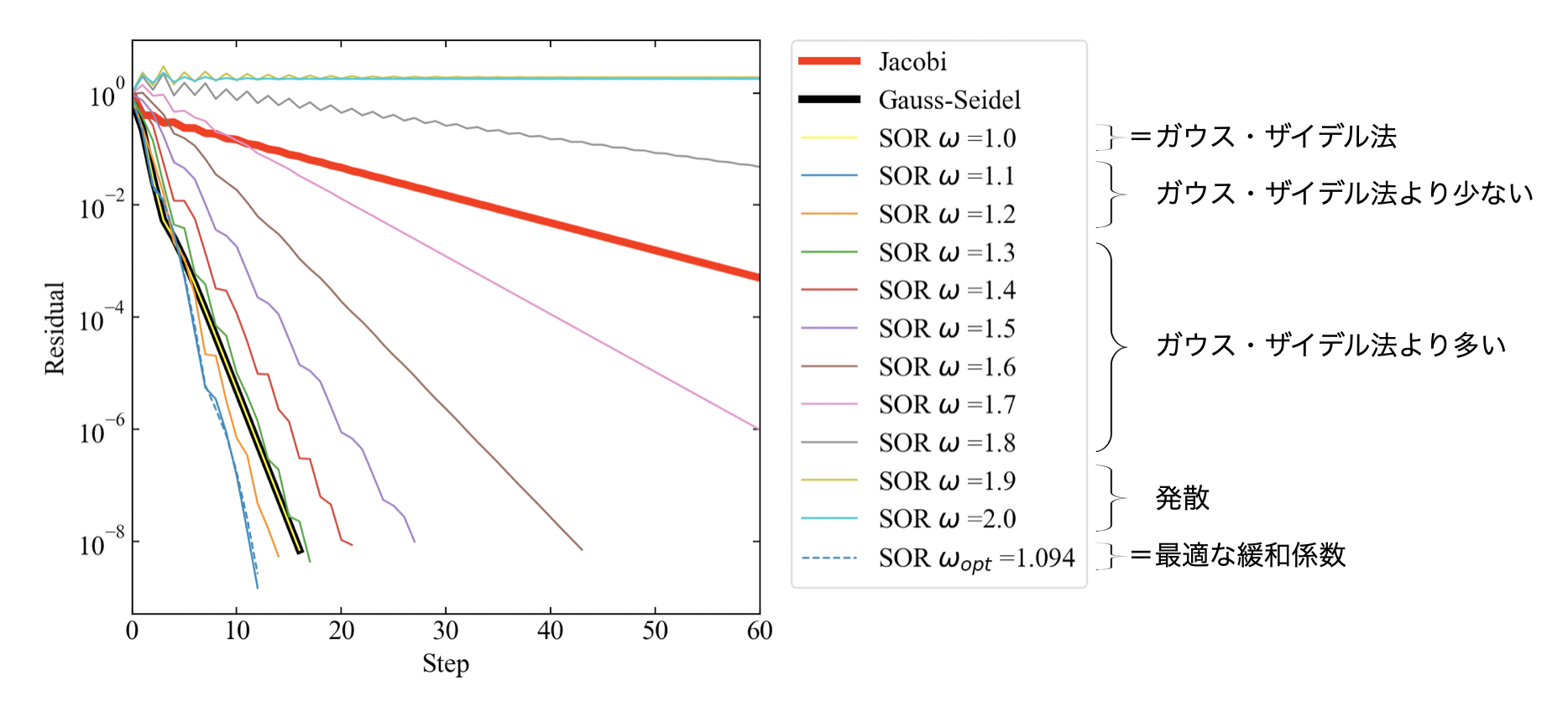
下図が結果です。緩和係数 $ω$ が1.0の時はガウス・ザイデル法と一致します。今回 $ω$ は1.0から2.0まで0.1刻みで振りましたが、この連立方程式の場合は $ω =$ 1.9, 2.0で発散（解がでたらめになる）するといった特徴もありました。

また最適な緩和係数の場合とパラスタで得られた $ω$ の値が近く、式（4）はしっかり実装できているのではと考えられます（文献があまりなかったので合っているか不安でした）。

まとめ

この記事ではSOR法の概要として漸化式と最適な緩和係数（加速パラメータ）を説明しました。最適な緩和係数は行列のスペクトル半径を使って求めるということで、固有値計算を使うことがわかりました。

筆者にとって線形代数は計算手法を覚えるということが主な学習方法でしたが、今回のスペクトル半径や固有値の関係性、行列操作の意味に重点を置いて学習するのも有用と感じました。

最後にSOR法をPythonで実装するコードを紹介しました。緩和係数にもよりますがこれまでのヤコビ法やガウス・ザイデル法よりも反復回数が削減できることがわかりました。

しかし、ヤコビ法は並列計算ができるという強みがあるので一概にどの手法が良いかは決まらないと思います。

参考文献

[1]:幸谷智紀, 連立一次方程式の解法2 -- 反復法 (2007), pp109

[2]:[線型代数] 特異値分解と低ランク近似

[3]:Varga, R. S. (2009). Matrix iterative analysis (Vol. 27). Springer Science & Business Media.

[4]:山崎郭滋, 偏微分方程式の数値解法入門, 森北出版,(2015), pp28

ヤコビ法、ガウス・ザイデル法、SOR法の3つを使えるようになりました！
Twitterでも関連情報をつぶやいているので、wat(@watlablog)のフォローお待ちしています！

連立方程式をSOR法で解くPythonコードと緩和係数のパラスタ

SOR法の概要

SOR法の漸化式

最適な緩和係数

SOR法で連立方程式を解くPythonコード

動作環境

Python環境

PC環境

まずは $ω$ を手入力

スペクトル半径から $ω_{o p t}$ を求めてパラスタ結果と比較する

最適な緩和係数を求める関数

検証用の全コード

まとめ

参考文献

コメントを残すコメントをキャンセル

最近の投稿

アーカイブ

カテゴリー

SOR法の概要

SOR法の漸化式

最適な緩和係数

SOR法で連立方程式を解くPythonコード

動作環境

Python環境

PC環境

まずはωを手入力

スペクトル半径からωoptを求めてパラスタ結果と比較する

最適な緩和係数を求める関数

検証用の全コード

まとめ

参考文献

SNSでもご購読できます。

コメントを残す コメントをキャンセル

最近の投稿

アーカイブ

カテゴリー

まずは $ω$ を手入力

スペクトル半径から $ω_{o p t}$ を求めてパラスタ結果と比較する

コメントを残すコメントをキャンセル